Eleanor Oldham, Senior Geophysicist
In Pressure Plot Basics I described the various components of a pressure plot covering a regional database. This is great for gaining regional insight into your data but is too much information when you’re trying to understand the likely column height of a prospective hydrocarbon accumulation. In the latter case it’s useful to create a separate pressure plot for each nearby well which samples the reservoir (and cap-rock) you’re evaluating.
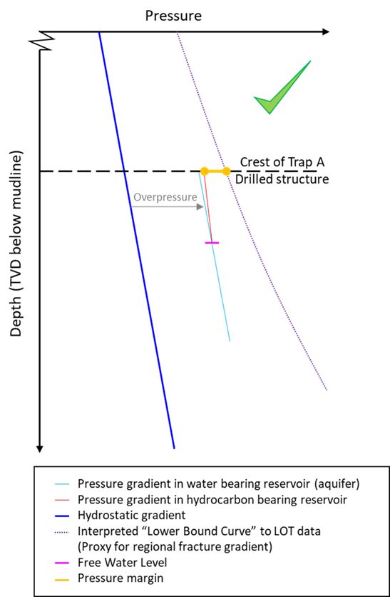
The cartoon above shows the aquifer and hydrocarbon gradients for one reservoir in one well. In this example I’ve assumed that we collected pressure data from both the water and hydrocarbon legs to give these gradients. The free water level (FWL) occurs at the intersection between the aquifer and hydrocarbon gradients (pink line).
If you only had pressure points from the hydrocarbon zone then a saturation height function could be used to work out where the FWL may be, given sufficient petrophysical data. Once we have the FWL, we can hang a water gradient off this point. This allows us to calculate how overpressured the aquifer is with respect to the hydrostatic gradient.
The aquifer and hydrocarbon gradients (from a well on structure) have been extrapolated upwards to the crest of Trap A (black dashed line). You’ll need to find the crestal depth from seismic mapping. At the crest, we can measure the differential between the hydrocarbon and fracture pressures to get the “pressure margin” (yellow bar). In Pressure Plot Basics we saw that a conservative fracture gradient (the “Lower Bound Curve”) could be interpreted from regional leak off test (LOT) data – the Lower Bound Curve (LBC) is the best proxy we can use for fracture gradient.
In this example, the yellow bar indicates a large, positive pressure margin: At the crest of Trap A, fracture pressure is much greater than the reservoir pressure (as measured in the hydrocarbon leg). This means we can be confident that the top-seal has not mechanically failed, given the overpressure of the reservoir and the height of the hydrocarbon column. The height of the hydrocarbon column has not been limited by the mechanical strength of the top seal.
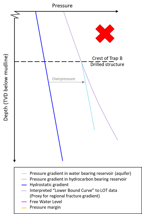
Overpressure has been increased in the second cartoon. When we extrapolate the aquifer gradient up to meet the crest of the Trap B, it meets the LBC: The pressure margin is zero. This suggests it is likely that the top-seal is at the point of mechanical failure. I say “likely” because the local fracture gradient could be quite different to the regionally defined LBC. In this scenario, the aquifer overpressure at Trap B is limited by the top-seal strength – any increase in pressure would be immediately vented to the overburden. Similarly, any hydrocarbons migrating into Trap B would be vented too. Trap B is therefore an example of a “blown trap”.
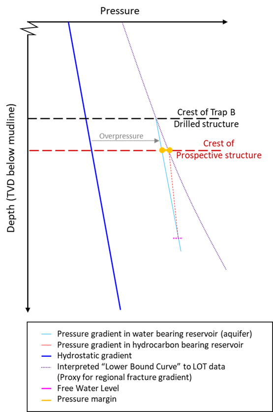
That helps us to understand what happened at the wells already drilled. But what about nearby prospects within (what we interpret to be) the same pressure cell? In the third cartoon I have added the crest of a nearby prospect to see how favourable the pressure margin is at that depth. The prospect is interpreted as belonging to the same pressure cell as Trap B, so we assume the same aquifer overpressure. We therefore measure a positive pressure margin at the crest of the prospect (yellow bar), suggesting the cap-rock above the prospect is capable of holding back a hydrocarbon column.
How long could that column be? To answer that question, we can drop down a hydrocarbon gradient from the LBC where it intersects the crestal depth of the prospect (red dashed line). The point at which this hydrocarbon gradient meets the aquifer gradient gives us the deepest possible FWL (pink dashed line). This is the longest possible hydrocarbon column that cap-rock could hold back before it suffers mechanical failure.
This prospect is an example of a “protected trap”. Trap B lies up-dip from the prospect and is at fracture pressure. Any pressure increases in this cell will be vented from Trap B, protecting any hydrocarbon columns in down-dip closures.
The assumptions we make when we use this method to evaluate a prospect are:
• Overpressure in the prospect is the same as the drilled well.
• The regional fracture gradient (defined using regional leak off test data) is appropriate here.
• We have accurately mapped the prospect’s depth from seismic.
In other words, the estimate on pressure margin (or column height) which we make for the prospect is subject to uncertainty. To account for all this uncertainty we can model distributions for all of the input parameters and combine these using Monte Carlo sampling. This can give us statistics such as the likelihood any hydrocarbon column is sustained at a prosect or the probability a trap is filled to spill. These statistics are useful when it comes to evaluating prospect risk and the likelihood of a achieving a minimum economic volume.
The same methodology can also be used for screening potential CCS sites, to understand how long a CO2 column a cap-rock will be able to hold-back before it fractures.
